PhysLab.net – Roller Coaster with Flight

This simulation shows a ball on a roller coaster where the ball can jump off the track. When the ball is on the track, it is colored blue; when in free flight it is colored red.
The spring is activated when the spring stiffness is non-zero, which you can change by clicking show controls. Clicking the spring on or spring off buttons also changes the spring stiffness. You can change parameters such as gravity or damping. Drag the ball with your mouse to change the starting position. If you don't see the simulation try instructions for enabling Java. Scroll down to see the math!

When Should the Ball Jump the Track?

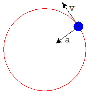
uniform circular motion

This simulation is based on the Roller Coaster with Spring and uses all of the physics described there. The main difference is that we check for when the ball should jump off the track into free flight. The key to when this happens lies in the formula for acceleration with uniform circular motion, which is

a = v²/r

(1)

This is the acceleration, a, needed to keep a projectile moving in a circle of radius r with velocity v. The direction of the acceleration is towards the center of the circle. So, moving faster in a given circle means you need more acceleration to stay on the same circle. Conversely, moving in a larger circle means you need less acceleration.

Suppose the ball is moving with velocity v over a hill shaped like a circle with radius r. The minimum acceleration (towards the center of the circle) needed to keep the ball on the hill is v²/r. If at any moment the acceleration (towards the center) is less than this, then the ball will fly off the hill.

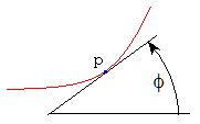
angle of tangent

To apply this to a general curve other than a circle, we need the notion of radius of curvature at a point p on the curve. Let φ = the angle of the tangent to the curve at p. We can express φ as φ = arctan(^dy⁄_dx) where ^dy⁄_dx is the slope of the curve at p. We define the curvature κ as the rate of change of the tangent angle φ as we move along the curve.

κ = ^dφ⁄_ds

(2)

where s = arc length along the curve. The radius of curvature r is the reciprocal of the curvature: r = ¹⁄_κ

We can estimate this using the table representing the curve. Here's how: for a given point p we estimate the slope a short distance δ on either side of p. Equation (2) is then approximated by

κ =	arctan(slope at p+δ) − arctan(slope at p−δ)
	2 δ

The radius of curvature r is then the reciprocal of this. And this radius of curvature is what we need to apply equation (1). We know that the ball will stay on the curve as long as the acceleration normal to the curve is greater than v²/r.

In the Simple Roller Coaster we developed an expression for the gravity force on the ball. In the Roller Coaster with Spring we developed an expression for the spring force on the ball. In those cases, we used the component of the force that was parallel to the track. Here, we want to know the component of the force that is perpendicular (normal) to the track. To determine the acceleration normal (perpendicular) to the curve we use the same calculations except that now we use sin θ instead of cos θ. F_gravity = m g sin θ
F_spring = c sin θ (√(s_x² + s_y²) − R) (Please see those pages for the definition of these symbols.) Since we already know cos θ from the Roller Coaster with Spring we can easily find sin θ from sin θ = √(1 − cos²θ) Now we can find the acceleration normal to the curve from F_gravity + F_spring = m a We then compare the acceleration to that given by equation (1) to determine whether the ball should leave the track. To stay on the track going over a hill, we must have a > v²/r. On the other hand, to stay on the track when going through a valley we need a < v²/r. (I am glossing over some details of how to determine the correct sign of the acceleration).

Switching to Free Flight

When the ball is on the track, the simulation is controlled by the differential equations given in the Roller Coaster with Spring. In this case there are two variables:

p = position on the track (measured by path length along the track)
v = velocity

When we detect that the ball should leave the track, we switch the controlling differential equations to those of "free flight". There are then four variables:

u_x = horizontal position
u_y = vertical position
v_x = horizontal velocity
v_y = vertical velocity

The differential equations for free flight are the same as those given for the 2-Dimensional Spring

Adjusting Velocity During Collision

While the ball is in free flight we need to handle collisions with the track. After a collision is detected (because the ball is below the track) we back up and use a binary search algorithm to get the simulation very close to the time of collision. The Colliding Blocks simulation has some more about collision handling in general.

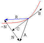
reflected velocity vector

Once the simulation has been run to very close to the time of collision, we need to adjust the velocity of the ball so that it bounces off the track. Define the following vectors (vectors are indicated by bold type):

A = (vx, vy) is the velocity vector of the ball
B = (1, k) is the vector tangent to the curve where slope = k
C = the component of A in the B direction
N = the component of A normal to B
R = the reflected velocity vector

Some elementary vector algebra gives us

C =	A · B	B
	B · B

N = A − C

R = C − N

(4)

The elasticity parameter determines how bouncy the ball is. Let e = elasticity. A perfectly elastic ball will have elasticity e = 1.0 and will bounce forever. An elasticity of e = 0.2 would indicate a rather "dead" ball that doesn't bounce very much. To model this behavior we multiply N in equation (4) by the elasticity to get R = C − e N This represents the new velocity that we assign to the ball at the time of collision.

Eventually, the ball will make smaller and smaller bounces. In real life, there comes a time when the ball is back in continuous contact with the ground. To determine whether the ball should "jump back onto the track" and be controlled by the "on the track" set of differential equations, we compare the magnitude of the normal vector e N to the magnitude of the total velocity vector. The test involves the stickiness parameter and looks like this:

if (	\|e N\|	< stickiness) then jump back onto track
	\|R\|

If the normal velocity e N is small enough we decide the ball should be back on the track. The stickiness is a parameter on the order of 0.1 that can be changed in the simulation controls.

Multiple Collisions

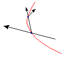
multiple collisions over one time step

The collision occurred as we were trying to advance the simulation a small time step (perhaps ¹⁄₁₀ of a second) from a certain time t₀ to the new current time t₁. Now that the collision has been handled, we attempt to run the simulation up to the current time t₁. If there are no new collisions detected, then this simulation step is done. However if a new collision is detected, we begin the entire collision handling process over again. We will eventually reach time t₁ even if we have to handle multiple collisions along the way.

The figure at left shows a typical situation where multiple collisions occur over one simulation time period because the ball goes into a tight corner at high speed.

Limitations of this Simulation

Unlike the other roller coaster simulations, this one does not have the option to use various tracks. The reason is that having a track that doesn't loop simplified the code considerably. For example, to determine whether there is a collision, we only test whether the ball is below the track. With a looped track there would be more complicated criteria for deciding if the ball has collided with the track, such as checking if it is inside or outside the track. So if you are looking for a programming project, grab the source code and go to work!