PhysLab.net – 2-Dimensional Spring

This simulation shows a single mass on a spring, which is connected to the ceiling. The mass is able to move in 2 dimensions, and gravity operates. Does the motion look random to you? Watch the graph for a while and you'll see its actually an intricate pattern.
You can change parameters in the simulation such as gravity, mass, spring stiffness, and friction (damping). You can drag the mass with your mouse to change the starting position. If you don't see the simulation try instructions for enabling Java. Scroll down to see the math!

Physics of the 2-Dimensional Spring

2D spring variables

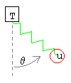
An immoveable (but draggable) anchor point has a spring and bob hanging below and swinging in two dimensions. Regard the bob as a point mass. Define the following variables:

θ = angle (0 = vertical, increases counter-clockwise)
S = spring stretch (displacement from rest length)
L = length of spring
u = position of bob
v = u'= velocity of bob
a = u''= acceleration of bob

Define some constants:

R = rest length of spring
T = position of anchor point
m = mass of bob
k = spring constant
b = damping constant
g = gravitational constant

i & j unit vectors

Note that for this simulation the vertical dimension increases downwards. We'll need the standard unit vectors i, j. We use bold and overline to indicate a vector.

i = unit vector in horizontal direction
j = unit vector in vertical (down) direction

There are three vector forces acting on the bob:

F_gravity = m g j = gravity acting straight down
F_spring = −k S (sin θ i + cos θ j) = the spring pulling (or pushing) along the line from bob to anchor point.
F_damping = −b (v_x i + v_y j) = damping (friction) acting opposite to the direction of motion of the bob, ie. opposite to its velocity vector.

Summing these forces and using Newton's second law we get: m a = F_gravity + F_spring + F_damping m (a_x i + a_y j) = m g j − k S (sin θ i + cos θ j) − b (v_x i + v_y j) We can write the horizontal and vertical components of the above as separate equations. This gives us two simultaneous equations. We also divide each side by m.

a_x = − ^k⁄_m S sin θ − ^b⁄_m v_x

(1a)

a_y = g − ^k⁄_m S cos θ − ^b⁄_m v_y

(1b)

These are the equations of motion. It only remains to show how S sin θ and S cos θ are functions of the position of the bob. The displacement of the spring S is the current length of the spring minus the rest length.

S = L − R

(2)

From the pythagorean theorem we can get the length of the spring L in terms of from the position of the bob, u, and the position of the anchor point, T.

$L = \sqrt{(u_x - T_x)^2 + (u_y - T_y)^2}$

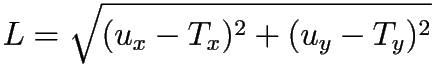
(3)

The sine and cosine of the angle θ are:

sin θ = (u_x − T_x)/L

(4a)

cos θ = (u_y − T_y)/L

(4b)

Numerical Solution of the 2-Dimensional Spring

To solve the equations of motion numerically, so that we can drive the simulation, we use the Runge-Kutta method for solving sets of ordinary differential equations. Since the Runge-Kutta method only works with first-order differential equations, we convert the two second-order equations (1) to the following four first-order equations. u_x' = v_x u_y' = v_y v_x' = − ^k⁄_m S sin θ − ^b⁄_m v_x v_y' = g − ^k⁄_m S cos θ − ^b⁄_m v_y Keep in mind that S sin θ and S cos θ are functions of the position of the bob, u_x, u_y, as given in equations (2-4).