PhysLab.net – Rigid Body Collisions

This simulation shows rectangular objects colliding in 2 dimensions.
Click near an object to exert a rubber band force with your mouse. With the keyboard you can control four "thrusters". The keys S,D,F,E control the blue object. The keys J,K,L,I (and also the arrow keys) control the green object. You can also set gravity, elasticity (bounciness), and damping (friction). You can choose from one to six objects. The mass of the green object is adjustable (the others are set to mass 1.0). If you don't see the simulation try instructions for enabling Java. Scroll down to see the math!

Here is a picture of how the keyboard controls are arranged. If the keys don't work, try clicking near an object first - this ensures that keystrokes are passed to the simulation instead of the buttons or scrollbars. On some browsers (Opera) you might have to also type into one of the numeric controls (like gravity) then click near an object before keystrokes are passed to the simulation.

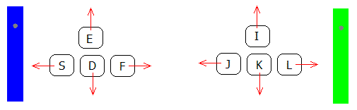
keyboard thruster controls

If elasticity is less than 1, and gravity is greater than zero, then the objects eventually settle onto the floor. Because this simulation does not implement resting contact the simulation will get 'stuck'.

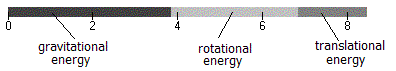
Energy Bar Graph

To check the correctness of the simulation, you can click the "show energy" checkbox and look at the display of the pre- and post-collision momentum and energy. If damping = 0 and elasticity = 1, then the energy should not change. The momentum should not change when objects collide, however it will change when an object collides with a wall (walls are assumed to be infinitely massive, so we don't model their movement).

The bar graph shows the gravitational, rotational and translational energy. Note that if gravity is zero, then there is no gravitational potential energy.

See the section on Energy and Momentum for how these quantities are calculated.

Physics Of Motion for Rigid Bodies

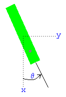
rigid body variables

Ignoring collisions for the moment, we develop the equations of motion for the objects. The forces on the objects are

Gravity
Friction
Thrust (keyboard controls)
Rubber band (mouse control)

For each body, there are three variables to specify position:

x = horizontal position of center of mass
y = vertical position of center of mass
θ = angle of rotation

In addition, each body has a velocity corresponding to each of these positions:

x' = v_x = horizontal velocity of center of mass
y' = v_y = vertical velocity of center of mass
θ' = ω = angular velocity

The equations of motion for the body involve the total force F = (F_x, F_y) and torque τ on the body as follows: F_x = m x''
F_y = m y''
τ = I θ'' where m = mass and I = moment of inertia about the center of mass (moment of inertia is defined in the next section). Note that we indicate vectors, such as F, with bold and an overline.

Thrust Force

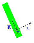
thrust force vector

We now build up the equations of motion by adding in one force at a time, beginning with the thrust force. Let T = (T_x, T_y) be the thrust force vector which operates at the point P on the body. The thrust force will accelerate the body according to m x'' = T_x
m y'' = T_y In these equations it doesn't matter where on the body the thrust force is applied. The point P can be anywhere on the body, yet because the body is rigid the thrust accelerates the entire body. On the other hand, for rotational movement it matters a great deal where on the body the thrust is applied.

Moment of inertia is the equivalent of mass for rotational physics. It measures how difficult it is to rotate a body about a given point. Since our rectangle bodies rotate freely about their center of mass, we use center of mass as the point for calculating moment of inertia. From a physics textbook you can find the equation for the moment of inertia about the center of a thin rectangular plate. It is given by I = m (width² + height²) ⁄ 12 Let R = (R_x, R_y) = be the distance vector from center of mass to P. The torque at the point P is given by the vector cross product R × T = R_x T_y − R_y T_x so we have I θ'' = R × T Actually torque is a vector, but since we are working in 2 dimensions we know that torque is always perpendicular to the plane and so we aren't using vector notation for it. The true vector cross product results in a vector. So the above cross product corresponds to the following 3 dimensional calculation: (R_x, R_y, 0) × (T_x, T_y, 0) = (0, 0, R_x T_y − R_y T_x) You can see that the result is always perpendicular to the plane, with zero x and y components. The general vector cross product of two vectors is defined as: (x, y, z) × (u, v, w) = (y w − z v, −x w + z u, x v − y u)

Rubber Band Force

The rubber band force in the simulation operates along the vector from point P on the body to the mouse position, call this vector L. The rubber band force is B = (B_x, B_y) = s L where s is the stretchiness constant. The treatment of this force is identical to the thrust force, so we add it in to get the following equations. m x'' = T_x + B_x
m y'' = T_y + B_y
I θ'' = R×T + R×B

Gravity Force

Let g = the gravitational constant. Gravity causes a force on the center of mass of −m g in the vertical direction leading to m y'' = T_y + B_y − m g Because gravity works on all points of the body, no torque is generated by gravity.

Damping Force

Damping (friction) causes a force opposite to the direction of motion. The faster you go, the more friction resists your motion. So the magnitude of the damping force is proportional to the velocity. Let k = the proportional damping constant. Adding this to our equations of motion gives

m x'' = T_x + B_x − k x'

(1)

m y'' = T_y + B_y − m g − k y'

(2)

I θ'' = R×T + R×B − k θ'

(3)

In a more realistic simulation, there may be different damping constants for rotational versus translational motion. But here, we use the same constant for both.

Equations (1-3) are the equations of motion for one of our rectangular bodies. As long as no collision occurs, these equations are in charge. Here is a recap of some of the variables:

m = mass
g = gravity constant
k = damping (friction) constant
T = thrust force vector
B = rubber band force vector
R = vector from center to point P where thrust is applied

Numerical Simulation

To use the Runge-Kutta method for solving a set of differential equations we need to convert the above 3 second order equations into 6 first order equations. Define the velocity variables

v_x = x' = horizontal velocity
v_y = y' = vertical velocity
ω = θ' = angular velocity

Then equations (1-3) become 6 first order differential equations x' = v_x
y' = v_y
θ' = ω
v_x' = (T_x + B_x − k v_x) ⁄ m
v_y' = (T_y + B_y − m g − k v_y) ⁄ m
ω' = (R × T + R × B − k ω) ⁄ I These equations are now in the form needed for solving numerically with the Runge-Kutta method. Each rectangle body will have its own set of 6 variables (3 positions x, y, θ and 3 velocities v_x, v_y, ω) and 6 first order differential equations.

How to Calculate Energy and Momentum

This section explains how the energy and momentum of the objects are calculated. See the description of the energy bar graph for how to observe these quantities in the simulation.

If there is no loss of energy to friction (damping = 0) or during collisions (elasticity = 1) then the energy of the system should not change.

A collision between objects should not change the angular momentum. However, a collision with a wall will not preserve angular momentum because the super massive walls are not included in the calculations of the momentum of the objects.

Gravitational energy is given by m g h where h = height of the object's center of mass above the floor.

Translational energy is ¹⁄₂ m v² where v is the velocity vector for the object's center of mass. Note that we use vector dot product to square the velocity vector.

Rotational energy is 1/2 I ω² where I is the moment of inertia and ω is the angular velocity.

Linear momentum in the horizontal direction is given by m v_x, in the vertical direction by m v_y.

Angular momentum is measured with regard to a particular point in space, for example the origin. It is given by: I ω k + m r × v where r is the distance vector from the origin to the object's center of mass. The vector k is the unit z vector, which points out of the x-y plane. You can see that the angular momentum has two components: the spinning component I ω k and the rotation about the origin given by the vector cross-product m r × v.

Collision Detection

At each step in the simulation, we check to see if there is a collision. The bodies can collide with each other or with a boundary wall. For the rectangular shapes we are using it is simple geometry to determine if a collision has occurred by checking if any vertex is within a wall or foreign body.

When a collision is detected, we use a binary search to back up the simulation to an earlier time just shortly before the collision occurred. We then make the approximation that the collision takes place at this exact time, and calculate the resulting changes in velocity as described below. The Colliding Blocks simulation further describes these aspects of collision handling.

Physics of Collision for Rigid Bodies in 2 Dimensions

Handling collisions is the most challenging part of this simulation. The explanation here is fairly condensed, so you may want to read some other descriptions as well.

Chris Hecker's Rigid Body Dynamics Information. See especially his article for Game Developer Magazine on Collision Response. Easy to read, with many other references listed on the web site. Unfortunately some of the PDF documents do not print their math correctly.
Physically Based Modeling is a set of course notes from Siggraph '97 by Andrew Witkin and David Baraff. See especially the sections on Rigid Body Dynamics. Fairly complete and rigorous explanations, but still quite readable. Covers the 3 dimensional case and also resting contact forces.
Physics For Game Developers by David M. Bourg (O'Reilly Press) has a section on linear and angular impulse on page 95, and resting contact forces on page 258. This book has good explanations, but often relies on hard-to-follow programming code to illustrate the physics.
The textbook Engineering Mechanics Dynamics by Robert Soutas-Little and Daniel Inman has relevant sections on Eccentric Impact.

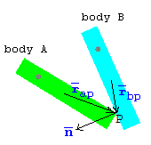
vectors involved in collision

Suppose a vertex on body A is colliding into an edge of body B at the point P. Define the following variables

m_a, m_b = mass of bodies A, B
r_ap = distance vector from center of mass of body A to point P
r_bp = distance vector from center of mass of body B to point P
ω_a1, ω_b1 = initial pre-collision angular velocity of bodies A, B
ω_a2, ω_b2 = final post-collision angular velocity of bodies A, B
v_a1, v_b1 = initial pre-collision velocities of center of mass bodies A, B
v_a2, v_b2 = final post-collision velocities of center of mass bodies A, B
v_ap1 = initial pre-collision velocity of impact point on body A
v_bp1 = initial pre-collision velocity of impact point on body B
n = normal (perpendicular) vector to edge of body B
e = elasticity (0 = inelastic, 1 = perfectly elastic)

We now use a standard formula for the velocity of an arbitrary point on a rotating and translating rigid body to get the pre-collision velocities of the points of collision (which is the point P on each body). v_ap1 = v_a1 + ω_a1 × r_ap
v_bp1 = v_b1 + ω_b1 × r_bp Similarly we have the final post-collision velocities v_ap2 and v_bp2 as v_ap2 = v_a2 + ω_a2 × r_ap
v_bp2 = v_b2 + ω_b2 × r_bp Here we are regarding the angular velocity as a 3 dimensional vector perpendicular to the plane, so that the cross product is calculated as ω × r = (0, 0, ω) × (r_x, r_y, 0) = (−ω r_y, ω r_x, 0) Now we can find an expression for the velocity with which the colliding points are approching each other. We call this the relative velocity. Let v_ab1 be the initial (pre-collision) relative velocity and v_ab2 be the final (post-collision) relative velocity. We define the relative velocities as follows v_ab1 = v_ap1 − v_bp1
v_ab2 = v_ap2 − v_bp2 Using the formulas given above for velocity of a point on a rigid body we can expand these to

v_ab1 = v_a1 + ω_a1 × r_ap − v_b1 − ω_b1 × r_bp

(4)

v_ab2 = v_a2 + ω_a2 × r_ap − v_b2 − ω_b2 × r_bp

(5)

Let the vector n be normal (perpendicular) to the edge of body B that is being impacted, and pointing outward from body B. Also let the vector n be of length 1. Then we can find the relative velocity in the direction of the normal n by using the dot product: relative normal velocity = v_ab1 · n = v_{ab1_x} n_x + v_{ab1_y} n_y Note that for a collision to occur this relative normal velocity must be negative (that is, the objects must be approaching each other). Let e be the elasticity of the collision, having a value between 0 (inelastic) and 1 (perfectly elastic). We now make an important assumption in the form of the following relation

v_ab2 · n = −e v_ab1 · n

(6)

This says that the velocity at which the objects fly apart is proportional to the velocity with which they were coming together. The proportionality factor is the elasticity e.

Collision Impulse

To resolve the collision, we will use the concept of an impulse. An impulse is the change in momentum of an object when a large force is applied over a very brief period of time. We imagine that during the collision there is a very large force acting for a very brief period of time. If you integrate (sum) that force over that brief time, you get the impulse.

Why do we need this strange concept of an impulse? Why not just use the familiar concept of force as in F = m a ? The answer is that we do not know what the forces are during the collision. With a supercomputer and some very complex software we could model the forces that occur during a collision. We would need to know details about the materials of the bodies, their exact geometry, how they deform under stress, how the stress propagates through the body, etc.

This is far beyond what our simple simulation can do. Luckily, we can assume that the collision happens so quickly that the position and orientation of the bodies do not change during the collision. Instead, all that changes is the velocities of the bodies. Since a change in velocity is a change in momentum (remember momentum = velocity times mass) we have the concept of an impulse.

We are assuming no friction for our collision, so the only force during the collision is in the direction perpendicular to the edge, which is given by the vector n. (Friction would cause a force parallel to the edge as well). Let the net impulse of the collision be j n where j is a parameter to be determined. Body A experiences an impulse of j n while body B experiences the equal but opposite impulse of −j n. The impulse is a change in momentum. Momentum has units of velocity times mass, so if we divide the impulse by the mass we get the change in velocity. We can relate pre- and post-collision velocities as

v_a2 = v_a1 + j n / m_a

(7)

v_b2 = v_b1 − j n / m_b

(8)

The change in angular momentum of body A from the impulse j n is given by r_ap × j n. You can think of the impulse as being applied at the point P, so it generates an instantaneous torque there. We then divide by the moment of inertia to convert the change in angular momentum to a change in angular velocity, so the post-collision angular velocities are

ω_a2 = ω_a1 + (r_ap × j n) / I_a

(9)

ω_b2 = ω_b1 − (r_bp × j n) / I_b

(10)

Solving for the Impulse Parameter

Now we can put all these various equations together and solve for the impulse parameter j. If you aren't interested in the details of solving the equations just skip down to the expression for j.

We start with equation (6), and then expand using our definition of relative velocity in equations (4-5). v_ab2 · n = −e v_ab1 · n
(v_ap2 − v_bp2) · n = −e v_ab1 · n
(v_a2 + ω_a2 × r_ap − v_b2 − ω_b2 × r_bp) · n = −e v_ab1 · n Let's expand the left hand side, using the impulse relationships in equations (7-10). ((v_a1 + j n / m_a) + (ω_a1 + (r_ap × j n) / I_a) × r_ap − (v_b1 − j n / m_b) − (ω_b1 − (r_bp × j n) / I_b) × r_bp) · n = −e v_ab1 · n We recognize that the left hand side contains the quantity v_ab1 · n as given by equation (4), so we move that to the right side. (j n / m_a + (r_ap × j n) × r_ap / I_a + j n / m_b + (r_bp × j n) ×r_bp / I_b) · n = −(1 + e) v_ab1 · n Note that n is assumed to be normalized so that n · n = 1. Also, to simplify the various vector products, we can use the triple scalar product rule (A × B) · C = (B × C) · A to derive the following identity (A × B) × A · B = (A × B) · (A × B) = (A × B)² (Here squaring a vector means taking its dot product with itself.) We can then simplify to j (1 / m_a + 1 / m_b + (r_ap × n)² / I_a + (r_bp × n)² / I_b) = −(1 + e) v_ab1 · n Dividing leads to our final expression for j.

j =	−(1 + e) v_ab1 · n
	¹⁄_{m_a} + ¹⁄_{m_b} + (r_ap × n)² ⁄ I_a + (r_bp × n)² ⁄ I_b

(11)

We can now calculate j at the time of collision using equation (11), and therefore calculate the post-collision velocities using the earlier equations (7-10).

We can use this same expression for calculating collisions with a wall by assuming that the mass of the wall is infinite. So let m_b → ∞ and I_b → ∞ and equation (11) becomes

j =	−(1 + e) v_ap1 · n
	¹⁄_{m_a} + (r_ap × n)² ⁄ I_a

Multiple Impacts

The above analysis only handles the case of a single corner and edge impact. There are several other simultaneous multiple impact cases, such as:

Two corners of object A impact a single wall
Two corners of object A impact object B
Two corners of object A impact different walls
Two corners of object A impact different objects

If there are simultaneous impacts among unrelated objects, these can be easily handled separately. For example, suppose objects A and B collide at the same time that objects C and D collide, then we can deal with each collision separately because they don't affect each other.

For the case of two adjacent corners of object A impacting either a single wall or another object's edge, we change the impact point to be the midpoint between the two corners and then handle it as other collisions.

The more complicated cases with corners of object A impacting different walls or multiple objects is not handled correctly by this simulation. What the code does is handle each impact separately, which will probably be wrong because these collisions are not independent.

Resting Contact

You will notice that certain settings of gravity and elasticity cause the simulation to eventually get stuck. Specifically, this happens when gravity > 0 and elasticity < 1. The problem occurs when an object is settling down onto the floor. The velocity of the object is becoming smaller with each collision because the elasticity is less than one. Eventually the velocity becomes so small that it can't keep gravity from pulling the object down past the floor. This is what results in the simulation getting 'stuck'.

The right thing to do at this point (which this simulation does not do) is recognize that the object is in resting contact with the floor. This would change the equations of motion for the object to include a contact force from the floor, which prevents the penetration of the object. See the Collisions With Contact simulation which handles this.